Barplots
vignette-barplots.RmdThe barplot panel allow to produce barplots using a variety of metadata (Fig. 1). As for the other panels this will only apply to the datasets, samples, ASV and taxa selected. Two major settings can be used:
Color according to taxonomy or according to ecological function (Fig. 1). Ecological function is according the list from Sommeria-Klein et al. (2021) as appears in their Supplementary material.
-
Variable to use
- fraction name
- ecosystem
- substrate
- depth (in m) and depth_level
- DNA_RNA
- latitude
- temperature
- salinity
- date (see below)
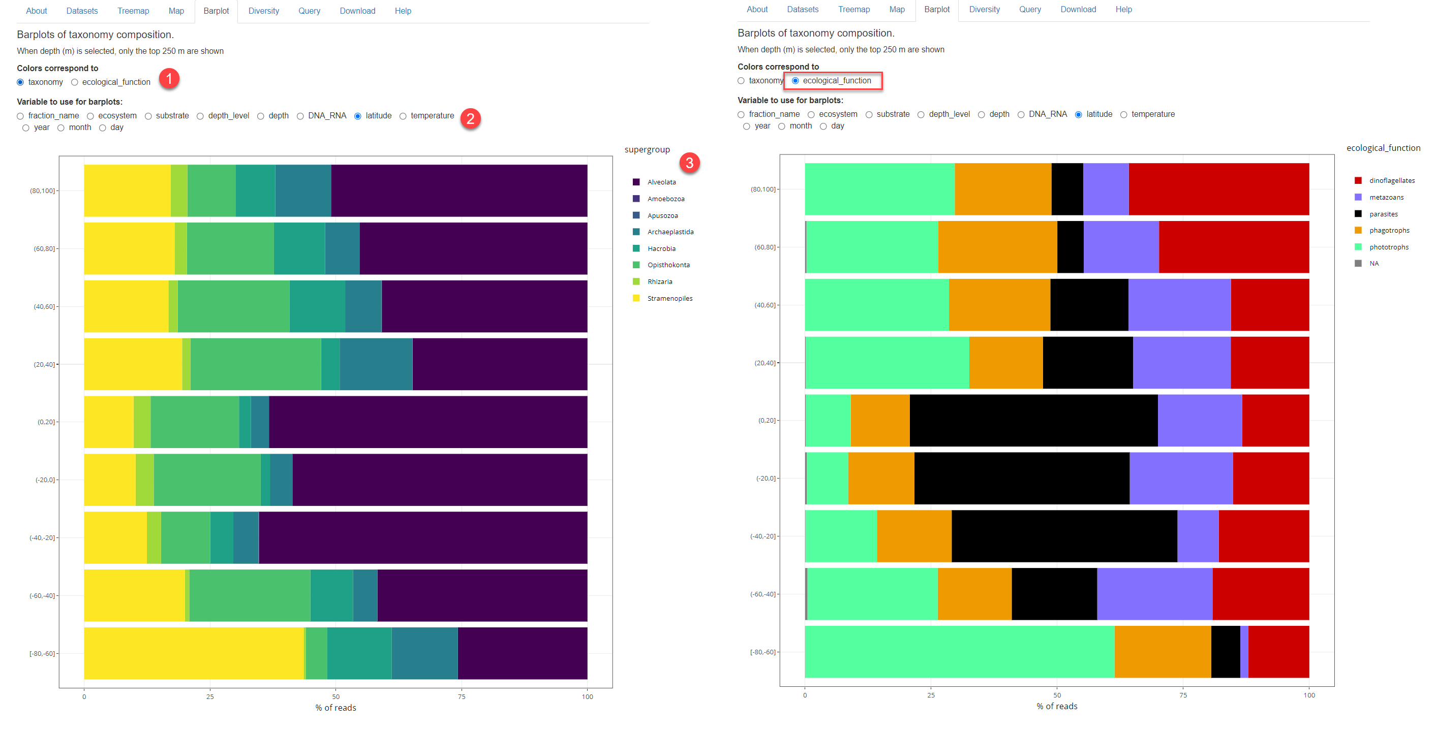
Fig. 1A: Barplot with taxonomy. 1: Color accoding to taxonomy or ecological function. 2: Variable to use. 3: Barplot. Left: Using taxonomy Right: using ecological function
The right side of the graph indicates, for each parameter range, the number of samples that fall into that range as well as the number of samples that contain the taxa selected.
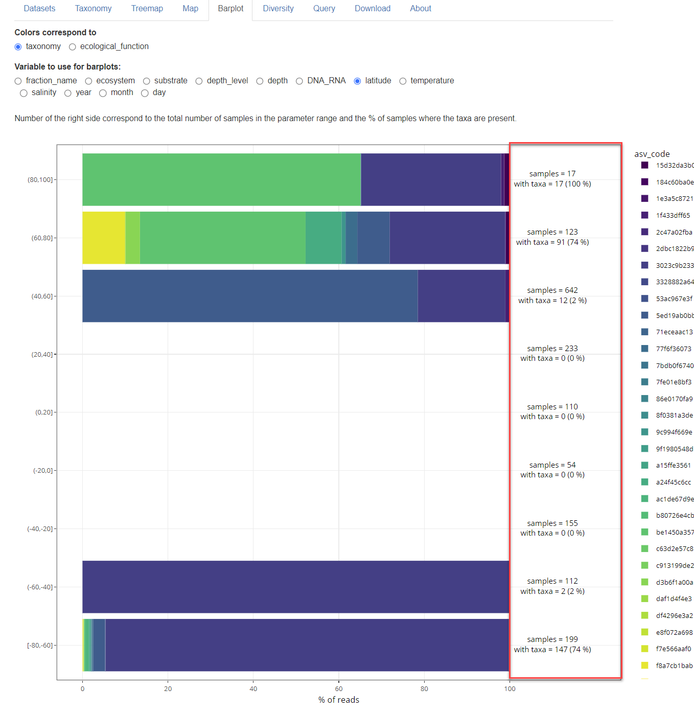
Fig. 1B: Number of samples and number of samples with taxa
Interactive plots
Plots are interactive and there is a menu on the upper right (Fig. 2). In particular you can isolate a specific taxonomic group by clicking on the group (Fig. 4).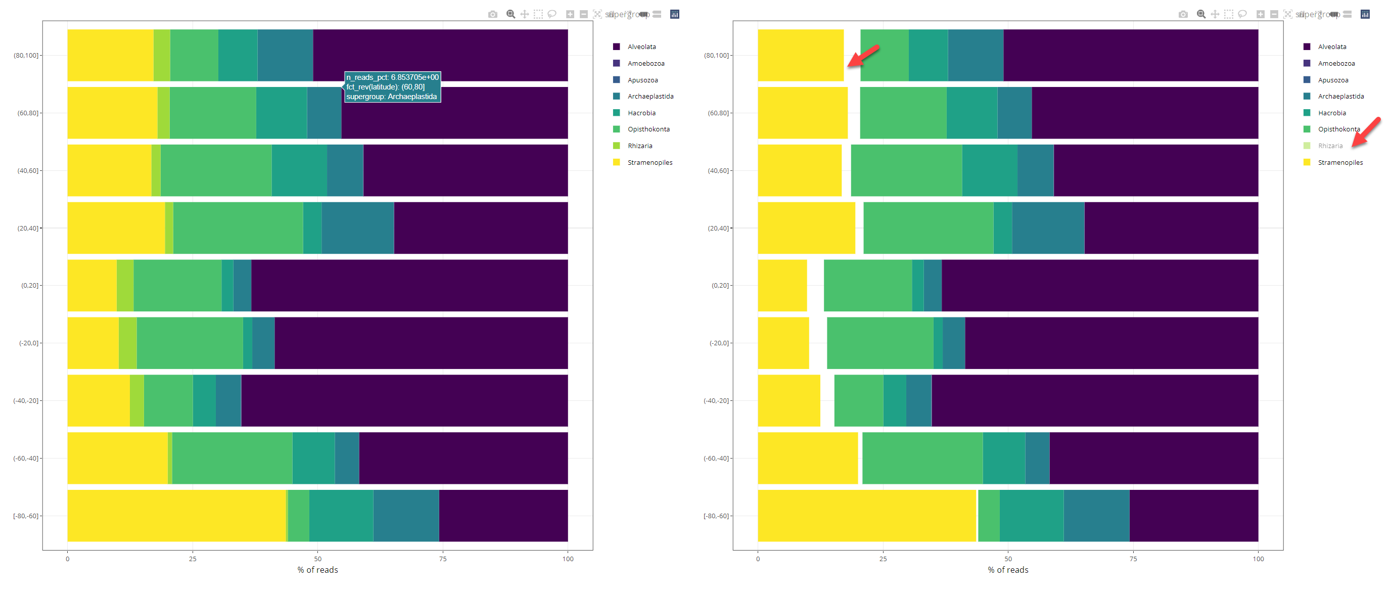
Fig. 2: Barplot interactive. Right: isolating a specific group.
Time series
Time series can also be plotted with data aggregated by:
- year (Fig. 3)
- month (Fig. 4)
- day
To test this feature it is best to use a single dataset (e.g. Spanish Blanes from Giner et al. 2019) and to use a single size fraction. Using the zoom function of plotly, one can more easily display monthly and daily data (Fig. 4).
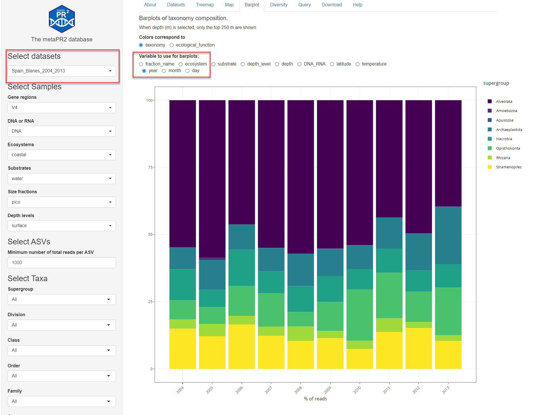
Fig. 3: Barplot time series with year aggregation
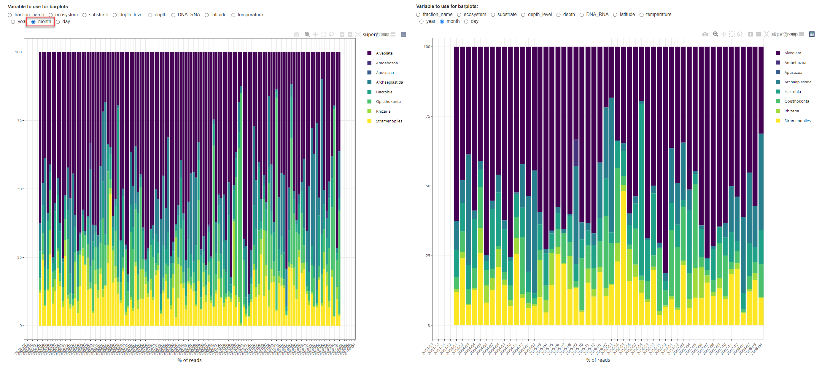
Fig. 4: Barplot time series with month aggregation. Right: after zooming
References
Sommeria-Klein, G., Watteaux, R., Ibarbalz, F.M., Pierella Karlusich, J.J., Iudicone, D., Bowler, C., Morlon, H., 2021. Global drivers of eukaryotic plankton biogeography in the sunlit ocean. Science 374, 594–599. https://doi.org/10.1126/science.abb3717
Giner, C.R., Balagué, V., Krabberød, A.K., Ferrera, I., Reñé, A., Garcés, E., Gasol, J.M., Logares, R., Massana, R., 2019. Quantifying long-term recurrence in planktonic microbial eukaryotes. Molecular Ecology 28, 923–935. https://doi.org/10.1111/mec.14929