The PR2 database is provided as a R package called pr2database. This page provides instruction to install and use the package.
Important Note. While the PR2 web interface provides access to the Ribosomal Operon Database sequences, this is not the case of the pr2database package that only provides access to 18S rRNA sequences.
Installation
- Requires R version 4.4
From GitHub
Install from the GitHub web site using the devtools package
if (!require("BiocManager", quietly = TRUE))
    install.packages("BiocManager")

BiocManager::install("Biostrings")

install.packages("devtools")
devtools::install_github("pr2database/pr2database")
* installing *source* package 'pr2database' ...
** R
** data
*** moving datasets to lazyload DB
** byte-compile and prepare package for lazy loading
** help
*** installing help indices
converting help for package 'pr2database'
finding HTML links ... fini
pr2 html
** building package indices
** testing if installed package can be loaded
*** arch - i386
*** arch - x64
* DONE (pr2database)
In R CMD INSTALLNote: You may have to install some packages required by pr2database if they are not installed on your machine
Launch shiny interface
pr2database::run_app()Analysing the database using R
Loading the database
The PR2 database is provided as a function that returns data frame (or a tibble). This is a join between the following tables:
- pr2_main
- pr2_taxonomy
- pr2_sequence
- pr2_metadata
- pr2_traits
- pr2_silva
- eukribo
- taxonomy_worms
- taxonomy_gbif
library("pr2database")

pr2 <- pr2_database()

# List of the different columns available - see the help of the package for information on each field

colnames(pr2)
#>  [1] "pr2_accession"                  "domain"
#>  [3] "supergroup"                     "division"
#>  [5] "subdivision"                    "class"
#>  [7] "order"                          "family"
#>  [9] "genus"                          "species"
#> [11] "genbank_accession"              "start"
#> [13] "end"                            "label"
#> [15] "gene"                           "organelle"
#> [17] "reference_sequence"             "added_version"
#> [19] "edited_version"                 "edited_by"
#> [21] "edited_remark"                  "remark"
#> [23] "taxo_id"                        "taxo_edited_version"
#> [25] "taxo_edited_by"                 "taxo_remark"
#> [27] "reference"                      "mixoplankton"
#> [29] "worms_id"                       "worms_marine"
#> [31] "worms_brackish"                 "worms_freshwater"
#> [33] "worms_terrestrial"              "seq_id"
#> [35] "sequence"                       "sequence_length"
#> [37] "ambiguities"                    "sequence_hash"
#> [39] "gb_date"                        "gb_division"
#> [41] "gb_definition"                  "gb_organism"
#> [43] "gb_organelle"                   "gb_taxonomy"
#> [45] "gb_strain"                      "gb_culture_collection"
#> [47] "gb_clone"                       "gb_isolate"
#> [49] "gb_isolation_source"            "gb_specimen_voucher"
#> [51] "gb_host"                        "gb_collection_date"
#> [53] "gb_environmental_sample"        "gb_country"
#> [55] "gb_lat_lon"                     "gb_collected_by"
#> [57] "gb_note"                        "gb_publication"
#> [59] "gb_authors"                     "gb_journal"
#> [61] "eukref_name"                    "eukref_source"
#> [63] "eukref_env_material"            "eukref_env_biome"
#> [65] "eukref_biotic_relationship"     "eukref_specific_host"
#> [67] "eukref_geo_loc_name"            "eukref_notes"
#> [69] "pr2_sample_type"                "pr2_sample_method"
#> [71] "pr2_latitude"                   "pr2_longitude"
#> [73] "pr2_depth"                      "pr2_ocean"
#> [75] "pr2_sea"                        "pr2_sea_lat"
#> [77] "pr2_sea_lon"                    "pr2_country"
#> [79] "pr2_location"                   "pr2_location_geoname"
#> [81] "pr2_location_geotype"           "pr2_location_lat"
#> [83] "pr2_location_lon"               "pr2_sequence_origin"
#> [85] "metadata_remark"                "pr2_continent"
#> [87] "pr2_country_geocode"            "pr2_country_lat"
#> [89] "pr2_country_lon"                "eukribo_UniEuk_taxonomy_string"
#> [91] "eukribo_V4"                     "eukribo_V9"
#> [93] "silva_taxonomy"                 "organelle_code"
#> [95] "species_url"
Install and load the libraries
The following examples makes use of the specifc R libraries
Install the libraries
install.packages("dplyr")      # For filtering the data
install.package("ggplot2")     # To plot data
install.package("maps")        # To plot maps

source("https://bioconductor.org/biocLite.R")  # This package is on Bioconductor
biocLite("Biostrings")         # To save fasta files
Load the libraries
Selecting sequences from a specific taxon
Let us select all the available sequences for the Mamiellophyceae Ostreococcus
  # Filter only the sequences for which the column genus contains Ostreococcus
pr2_ostreo <- pr2 %>%
  dplyr::filter(genus == "Ostreococcus")

  # Select only the columns of interest
  pr2_ostreo <- pr2_ostreo %>%
    dplyr::select( genbank_accession, species,
                    pr2_sample_type, gb_strain, gb_clone,
                    pr2_latitude, pr2_longitude,
                    sequence_length, sequence, reference_sequence,
                    eukribo_UniEuk_taxonomy_string)

  pr2_ostreo
#> # A tibble: 294 × 11
#>    genbank_accession species     pr2_sample_type gb_strain gb_clone pr2_latitude
#>    <chr>             <chr>       <chr>           <chr>     <chr>           <dbl>
#>  1 AF525872          Ostreococc… environmental   NA        UEPACIp5         NA
#>  2 EU562149          Ostreococc… environmental   NA        IND2.6           NA
#>  3 AY425309          Ostreococc… environmental   NA        RA01041…         NA
#>  4 GQ426346          Ostreococc… culture         CB6       NA               NA
#>  5 KC583118          Ostreococc… environmental   NA        RS.12f.…         NA
#>  6 JN862906          Ostreococc… culture         BCC48000  NA               NA
#>  7 JQ692065          Ostreococc… environmental   NA        PUPF_60         -43.3
#>  8 FR874749          Ostreococc… environmental   NA        1815F12          60.3
#>  9 FJ431431          Ostreococc… environmental   NA        RA07100…         NA
#> 10 EU561670          Ostreococc… environmental   NA        IND1.11         -35.0
#> # ℹ 284 more rows
#> # ℹ 5 more variables: pr2_longitude <dbl>, sequence_length <int>,
#> #   sequence <chr>, reference_sequence <int>,
#> #   eukribo_UniEuk_taxonomy_string <chr>
Exporting the sequences to fasta
We will save the Ostreococcus sequences to a FASTA file. This is easy done with the bioconductor package BioStrings.
  # Importing the sequence in a Biostring set

  seq_ostreo <- Biostrings::DNAStringSet(pr2_ostreo$sequence)

  # Constructing the name of each sequecne (the first line of the fasta file)
  # using the genbank accession, species name, strain name and clone name

  names(seq_ostreo) <- paste(pr2_ostreo$genbank_accession, pr2_ostreo$species,
                             "strain",pr2_ostreo$gb_strain,
                             "clone",pr2_ostreo$gb_clone,
                              sep="|")

  # Displaying the Biostring set
  seq_ostreo
#> DNAStringSet object of length 294:
#>       width seq                                             names
#>   [1]  1766 ACCTGGTTGATCCTGCCAGTAG...AGGTGAACCTGCAGAAGGATCA AF525872|Ostreoco...
#>   [2]   836 AAAGCTCGTAGTCGGATTTTGG...TCTGGGCCGCACGCGCGCTACA EU562149|Ostreoco...
#>   [3]  1728 GCCAGTAGTCATATGCTTGTCT...GAGAAGTCGTAACAAGGTTTCC AY425309|Ostreoco...
#>   [4]  1652 AGCCATGCATGTCTAAGTATAA...TGGATTACCGTGGGAAATTCGT GQ426346|Ostreoco...
#>   [5]  1764 CCTGGTTGATCCTGCCAGTAGT...TAGGTGAACCTGCAGAAGGATC KC583118|Ostreoco...
#>   ...   ... ...
#> [290]   672 GCTCGTAGTCGGACTTTGGCTG...TAGTTGGTGGAGTGATTTGTCT KT860809|Ostreoco...
#> [291]   540 ATAGCGTATATTTAAGTTGTTG...AAGGCTGAAACTTAAAGGAATT AY465412|Ostreoco...
#> [292]   540 ATAGCGTATATTTAAGTTGTTG...AAGGCTGAAACTTAAAGGAATT AY465413|Ostreoco...
#> [293]   540 ATAGCGTATATTTAAGTTGTTG...AAGGCTGAAACTTAAAGGAATT AY465414|Ostreoco...
#> [294]  1760 CCTGGTTGATCCTGCCAGTAGT...TCCGTAGGTGAACCTGCGGAAG CAID01000012|Ostr...

  # Saving the sequences as a fasta file
  Biostrings::writeXStringSet(seq_ostreo, "examples/pr2_ostreo.fasta", width = 80)
The fasta file will look as follows
>AF525872|Ostreococcus_lucimarinus|strain|NA|clone|UEPACIp5
ACCTGGTTGATCCTGCCAGTAGTCATATGCTTGTCTCAAAGATTAAGCCATGCATGTCTAAGTATAAGCGTTATACTGTG
AAACTGCGAATGGCTCATTAAATCAGCAATAGTTTCTTTGGTGGTGTTTACTACTCGGATAACCGTAGTAATTCTAGAGC
TAATACGTGCGTAAATCCCGACTTCGGAAGGGACGTATTTATTAGATAAAGACCG...
>EU562149|Ostreococcus_lucimarinus|strain|NA|clone|IND2.6
AAAGCTCGTAGTCGGATTTTGGCTGAGAACGGTCGGTCCGCCGTTAGGTGTGCACTGACTGGTCTCAGCTTCCTGGTGAG
GAGGTGTGCTTCATCGCCACTTAGTCACCGTGGTTACTTTGAAAAAATTAGAGTGTTCAAAGCGGGCTTACGCTTGAATA
TATTAGCATGGAATAACACCATAGGACTCCTGTCCTATTTCGTTGGTCTCGGGACGGGAGTAATGATTAAGATGAACAGT
TGGGGGCATTCGTATTTCATTGTCAGAGGTGAAATTCTTGGATTT...
>AY425309|Ostreococcus_lucimarinus|strain|NA|clone|RA010412.39
GCCAGTAGTCATATGCTTGTCTCAAAGATTAAGCCATGCATGTCTAAGTATAAGCGTTATACTGTGAAACTGCGAATGGC
TCATTAAATCAGCAATAGTTTCTTTGGTGGTGTTTACTACTCGGATAACCGT...
Doing an histogram of the sequence length
  ggplot(pr2_ostreo) +
    geom_histogram(aes(sequence_length), binwidth = 50, fill="blue") +
    xlim(0,2000) + xlab("Sequence length") + ylab("Number of sequences") +
    ggtitle("Ostreococcus sequences")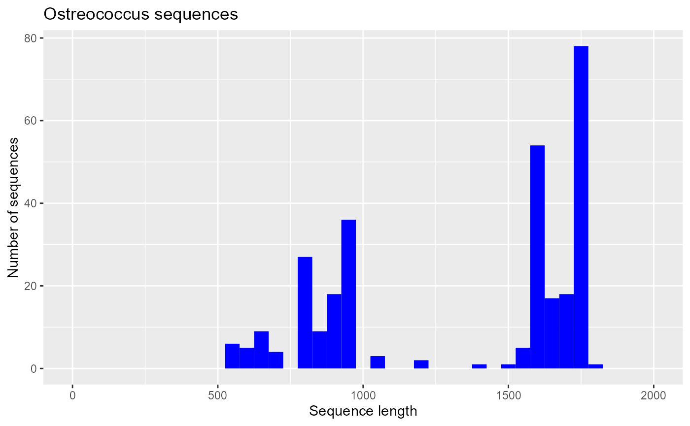
Drawing a map of sequence locations
  library(maps)
  world <- map_data("world")

  ggplot() +
    geom_polygon(data = world, aes(x=long, y = lat, group = group), fill="grey") +
    coord_fixed(1.3) +
    geom_point(data=pr2_ostreo, aes(x=pr2_longitude, y=pr2_latitude), fill="blue", size=2, shape=21) +
    ggtitle("Ostreococcus")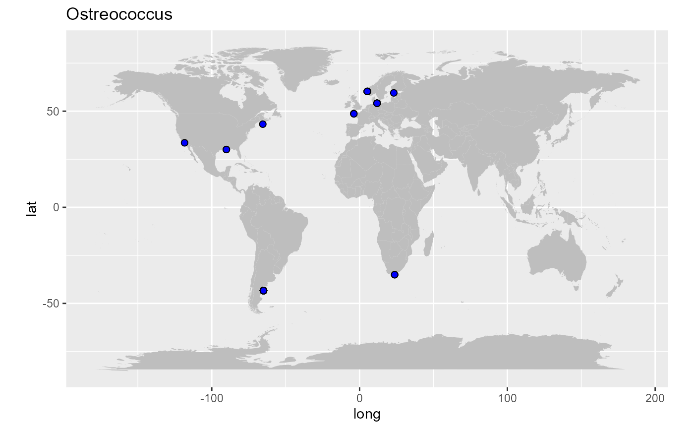
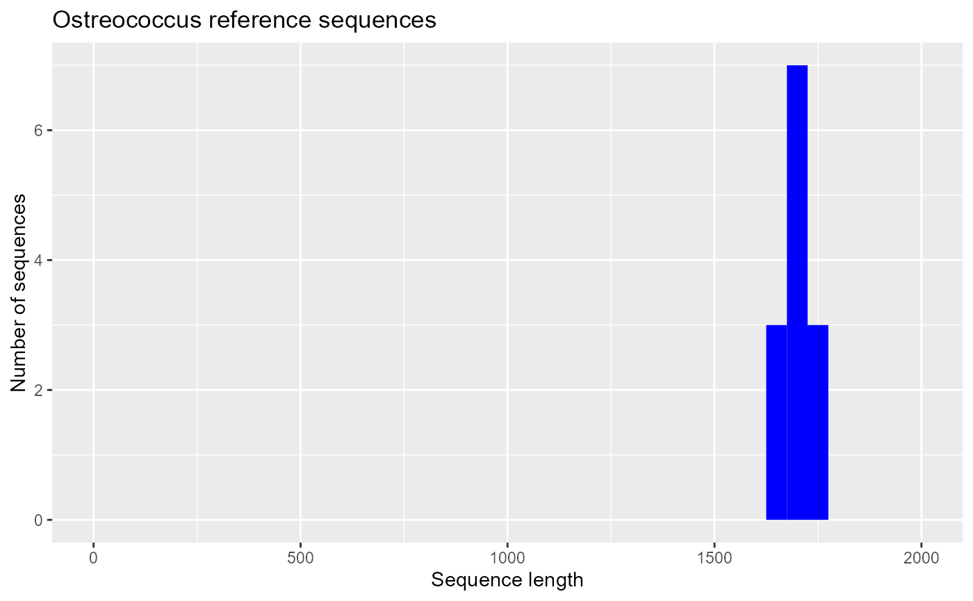
Selecting reference sequences
Reference sequences are a subset of sequences that are representative of the major taxa in a group. Usually they are long sequences and can be used to build a reference alignment (compare the histogram of reference to that all PR2 sequences).
 pr2_ostreo_reference <- pr2_ostreo %>%
  filter(reference_sequence == 1)

  pr2_ostreo_reference
#> # A tibble: 32 × 11
#>    genbank_accession species     pr2_sample_type gb_strain gb_clone pr2_latitude
#>    <chr>             <chr>       <chr>           <chr>     <chr>           <dbl>
#>  1 AF525872          Ostreococc… environmental   NA        UEPACIp5           NA
#>  2 JN862906          Ostreococc… culture         BCC48000  NA                 NA
#>  3 AY425308          Ostreococc… culture         RCC 356   1                  NA
#>  4 AF525852          Ostreococc… environmental   NA        UEPACDp1           NA
#>  5 AF525858          Ostreococc… environmental   NA        UEPAC30…           NA
#>  6 AF525857          Ostreococc… environmental   NA        UEPAC05…           NA
#>  7 AF525861          Ostreococc… environmental   NA        UEPACGp3           NA
#>  8 AF525848          Ostreococc… environmental   NA        UEPACAp1           NA
#>  9 AF525859          Ostreococc… environmental   NA        UEPAC30…           NA
#> 10 AF525855          Ostreococc… environmental   NA        UEPACXp1           NA
#> # ℹ 22 more rows
#> # ℹ 5 more variables: pr2_longitude <dbl>, sequence_length <int>,
#> #   sequence <chr>, reference_sequence <int>,
#> #   eukribo_UniEuk_taxonomy_string <chr>

  ggplot(pr2_ostreo_reference) +
  geom_histogram(aes(sequence_length), binwidth = 50, fill="blue") +
  xlim(0,2000) + xlab("Sequence length") + ylab("Number of sequences") +
  ggtitle("Ostreococcus reference sequences")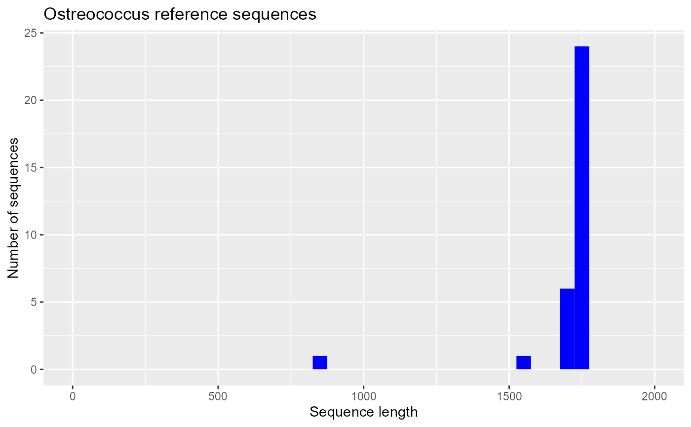
Selecting sequences annotated in the EukRibo database
EukRibo is a high quality 18S reference database (Berney et al. 2022)
 pr2_ostreo_eukribo <- pr2_ostreo %>%
  filter(!is.na(eukribo_UniEuk_taxonomy_string))

  pr2_ostreo_eukribo
#> # A tibble: 13 × 11
#>    genbank_accession species     pr2_sample_type gb_strain gb_clone pr2_latitude
#>    <chr>             <chr>       <chr>           <chr>     <chr>           <dbl>
#>  1 GQ426347          Ostreococc… culture         BCC40000d NA                 NA
#>  2 AY425308          Ostreococc… culture         RCC 356   1                  NA
#>  3 JN862916          Ostreococc… culture         BCC69000  NA                 NA
#>  4 AB058376          Ostreococc… culture         MBIC10636 NA                 NA
#>  5 AY425311          Ostreococc… culture         RCC 393   NA                 NA
#>  6 AY425310          Ostreococc… culture         RCC 143   NA                 NA
#>  7 JN862917          Ostreococc… culture         BCC7000   NA                 NA
#>  8 GQ426331          Ostreococc… culture         BCC1000   NA                 NA
#>  9 AY425313          Ostreococc… culture         RCC 501   NA                 NA
#> 10 AY329635          Ostreococc… NA              NA        NA                 NA
#> 11 JN862915          Ostreococc… culture         BCC68000  NA                 NA
#> 12 AY329636          Ostreococc… NA              NA        NA                 NA
#> 13 AY425307          Ostreococc… culture         RCC 344   NA                 NA
#> # ℹ 5 more variables: pr2_longitude <dbl>, sequence_length <int>,
#> #   sequence <chr>, reference_sequence <int>,
#> #   eukribo_UniEuk_taxonomy_string <chr>

  ggplot(pr2_ostreo_eukribo) +
  geom_histogram(aes(sequence_length), binwidth = 50, fill="blue") +
  xlim(0,2000) + xlab("Sequence length") + ylab("Number of sequences") +
  ggtitle("Ostreococcus sequences annotated in EukRibo")