PR2 - Mixoplankton database

Daniel Vaulot

The Mixoplankton Database (MDB, DOI 10.5281/zenodo.7560582) has been developed by Mitra et al. 2023 (https://doi.org/10.1111/jeu.12972).

It tabulates species that belong to the mixoplankton. This database has been linked to the PR database which contains a new field called mixoplankton

Values for this field are as follows:

• CM - Constitutive Mixoplankton
• GNCM - Generalist Non-Constitutive Mixoplankton
• pSNCM - plastidic Specialist Non-Constitutive Mixoplankton
• eSNCM - endosymbiotic Specialist Non-Constitutive Mixoplankton

In this small tutorial we explain how to access mixoplankton sequences from PR2.

Reference

• Mitra, Aditee, David A. Caron, Emile Faure, Kevin J. Flynn, Suzana Gonçalves Leles, Per J. Hansen, George B. McManus, et al. 2023. « The Mixoplankton Database – Diversity of Photo-Phago-Trophic Plankton in Form, Function and Distribution across the Global Ocean ». Journal of Eukaryotic Microbiology : e12972. https://doi.org/10.1111/jeu.12972.

# Loading the necessary packages

  library("ggplot2")
  library("dplyr")
  library("tidyr")
  library("DT")
  library("forcats")
  library("stringr")
  library("treemapify")
  library(patchwork)

  library("pr2database")
  packageVersion("pr2database")
#> [1] '5.0.0'

# Read the PR2 database
  
  pr2 <- pr2_database() %>% 
  # Only keep 18S (do not consider plastids)
    filter(gene == "18S_rRNA")

Extracting from PR2 the mixoplankton sequences

  pr2_mixopk <- pr2 %>% 
  # Remove sequences for which we have no taxonomy from Silva
    filter(!is.na(mixoplankton))
  

Total number of PR2 sequences belonging to mixoplankton : 3517

table <- pr2_mixopk %>% 
  count(mixoplankton)

DT::datatable(table, 
             caption="Number of sequences for each type of mixoplankton.", 
             rownames = FALSE)

table <- pr2_mixopk %>% 
  select(species, mixoplankton) %>% 
  distinct() %>% 
  count(mixoplankton)

DT::datatable(table, 
             caption="Number of species for each type of mixoplankton.", 
             rownames = FALSE)

Number of sequences of mixoplankton for each type at genus level

# Define a function for treemaps

pr2_treemap <- function(pr2, level1, level2) {
  # Group
  pr2_class <- pr2 %>%
    count(mixoplankton, {{level1}},{{level2}}) %>% 
    filter(!is.na({{level2}})) %>%
    ungroup()

  # Do a treemap
  
  ggplot(pr2_class, aes(area = n, fill = {{level2}}, 
                        subgroup = {{level1}}, label = {{level2}})) +
           treemapify::geom_treemap()
  
  ggplot(pr2_class, aes(area = n, fill= {{level1}}, 
                        subgroup = {{level1}}, label = {{level2}})) +
    treemapify::geom_treemap() +
    treemapify::geom_treemap_text(colour = "white", 
                                  place = "centre", grow = TRUE) +
    treemapify::geom_treemap_subgroup_border() +
    treemapify::geom_treemap_subgroup_text(place = "centre", grow = T, 
                                           alpha = 0.5, colour = "black", 
                                           min.size = 0) +
    theme_bw() +
    scale_color_brewer() +
    guides(fill = FALSE) +
    facet_wrap(~ mixoplankton, ncol=2)
}

  g1 <- pr2_treemap(pr2_mixopk, subdivision, genus) +
    labs(title = "PR2 mixoplankton")

  g1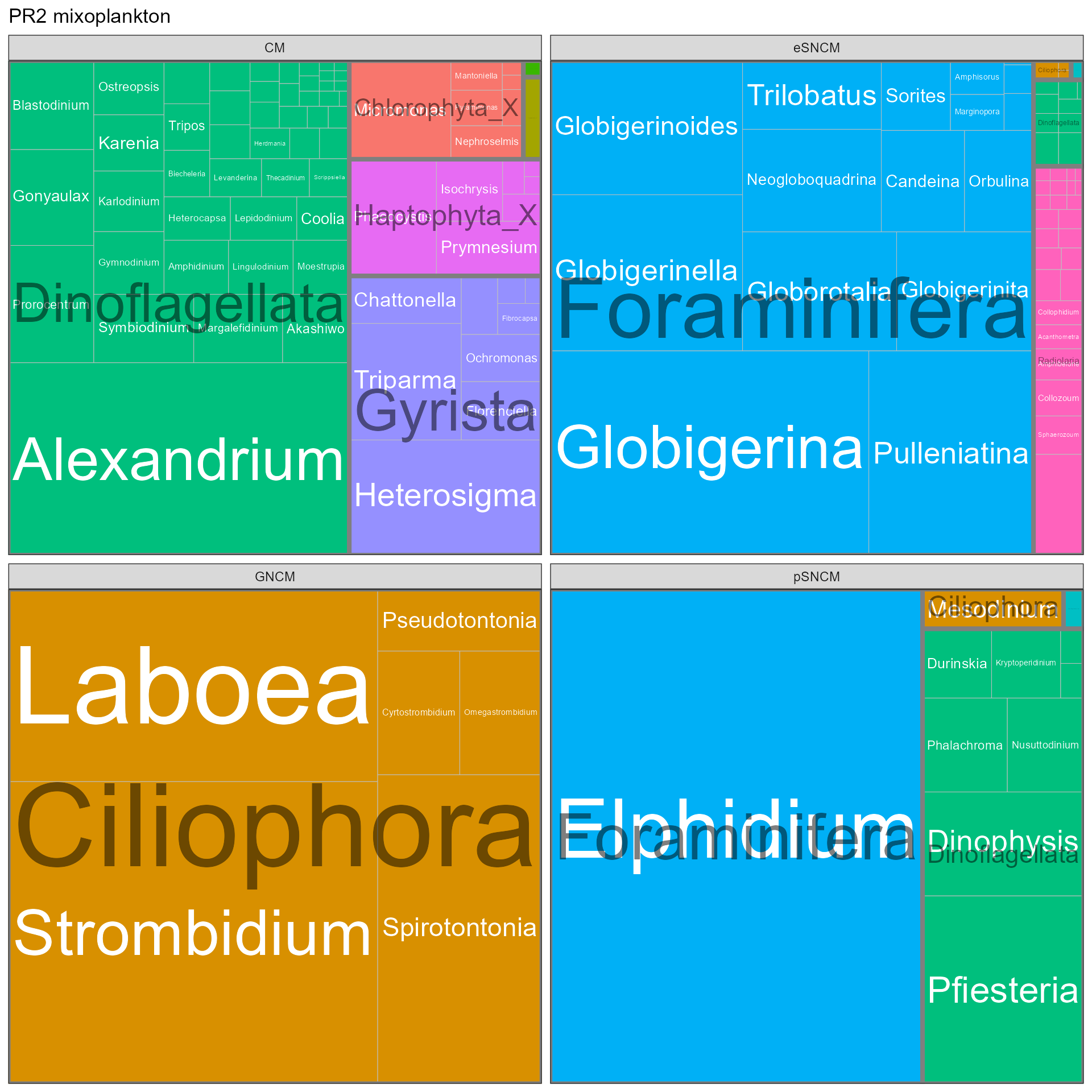

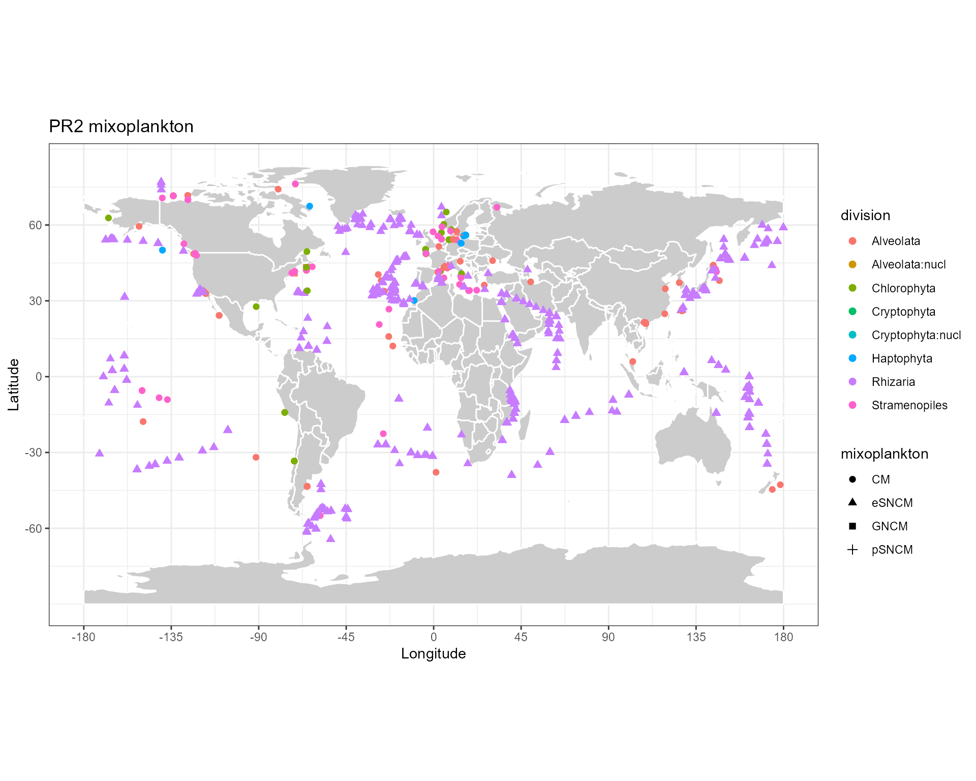
Localisation of mixoplankton sequences

map_get_world <- function(resolution="coarse"){
  # Change to "coarse" for global maps / "low" for regional maps
  worldMap <- rworldmap::getMap(resolution = resolution)
  world.points <- fortify(worldMap)
  world.points$region <- world.points$id
  world.df <- world.points[,c("long","lat","group", "region")]
  }


map_world <- function(color_continents = "grey80", 
                      color_borders = "white", 
                      resolution = "coarse") {

  # Background map using the maps package
  # world.df <- map_data("world")

  world.df <- map_get_world(resolution)

  map <- ggplot() +
    geom_polygon(data = world.df, 
                 aes(x=long, y = lat, group = group), 
                 fill=color_continents, 
                 color=color_borders) +
    # scale_fill_manual(values= color_continents , guide = FALSE) +
    scale_x_continuous(breaks = (-4:4) * 45) +
    scale_y_continuous(breaks = (-2:2) * 30) +
    xlab("Longitude") + ylab("Latitude") +
    coord_fixed(1.3) +
    theme_bw()
    # species_map <- species_map + coord_map ()  # Mercator projection
    # species_map <- species_map + coord_map("gilbert") # Nice for the poles
  return(map)
  }

 map_world() + 
  geom_point(data=pr2_mixopk, 
             aes(x=pr2_longitude, y=pr2_latitude, color=division, shape = mixoplankton), 
             size=2) +
  ggtitle("PR2 mixoplankton")