  library("ggplot2")
  library("dplyr")
  library("knitr")
  library("forcats")
  library("stringr")
  library("rworldmap")
  library("treemapify")
  library("pr2database")

  packageVersion("pr2database")
#> [1] '5.1.0'

  pr2 <- pr2_database()

  pr2_photo <- pr2 %>%
    filter((division %in% c("Chlorophyta", "Dinophyta",
                           "Cryptophyta",
                           "Haptophyta", "Ochrophyta")) &
          !(class %in% c("Syndiniales", "Sarcomonadea")))
  pr2_ref <- pr2 %>% filter(!is.na(reference_sequence))
PR2 fields
colnames(pr2)
#>   [1] "pr2_main_id"                    "pr2_accession"
#>   [3] "domain"                         "supergroup"
#>   [5] "division"                       "subdivision"
#>   [7] "class"                          "order"
#>   [9] "family"                         "genus"
#>  [11] "species"                        "genbank_accession"
#>  [13] "start"                          "end"
#>  [15] "label"                          "gene"
#>  [17] "organelle"                      "taxo_id"
#>  [19] "species_version_5.0"            "reference_sequence"
#>  [21] "remark"                         "mixoplankton"
#>  [23] "HAB_species"                    "ecological_function"
#>  [25] "worms_id"                       "worms_marine"
#>  [27] "worms_brackish"                 "worms_freshwater"
#>  [29] "worms_terrestrial"              "gbif_id"
#>  [31] "sequence"                       "sequence_length"
#>  [33] "ambiguities"                    "sequence_hash"
#>  [35] "gb_date"                        "gb_division"
#>  [37] "gb_definition"                  "gb_organism"
#>  [39] "gb_organelle"                   "gb_taxonomy"
#>  [41] "gb_strain"                      "gb_culture_collection"
#>  [43] "gb_clone"                       "gb_isolate"
#>  [45] "gb_isolation_source"            "gb_specimen_voucher"
#>  [47] "gb_host"                        "gb_collection_date"
#>  [49] "gb_environmental_sample"        "gb_country"
#>  [51] "gb_lat_lon"                     "gb_collected_by"
#>  [53] "gb_note"                        "gb_sequence"
#>  [55] "gb_publication"                 "gb_authors"
#>  [57] "gb_journal"                     "eukref_name"
#>  [59] "eukref_source"                  "eukref_env_material"
#>  [61] "eukref_env_biome"               "eukref_biotic_relationship"
#>  [63] "eukref_specific_host"           "eukref_geo_loc_name"
#>  [65] "eukref_notes"                   "pr2_sample_type"
#>  [67] "pr2_sample_method"              "pr2_latitude"
#>  [69] "pr2_longitude"                  "pr2_depth"
#>  [71] "pr2_ocean"                      "pr2_sea"
#>  [73] "pr2_sea_lat"                    "pr2_sea_lon"
#>  [75] "pr2_country"                    "pr2_location"
#>  [77] "pr2_location_geoname"           "pr2_location_geotype"
#>  [79] "pr2_location_lat"               "pr2_location_lon"
#>  [81] "pr2_sequence_origin"            "pr2_size_fraction"
#>  [83] "metadata_remark"                "pr2_continent"
#>  [85] "pr2_country_geocode"            "pr2_country_lat"
#>  [87] "pr2_country_lon"                "eukribo_UniEuk_taxonomy_string"
#>  [89] "eukribo_V4"                     "eukribo_V9"
#>  [91] "silva_taxonomy"                 "organelle_code"
#>  [93] "species_rod"                    "infraspecific_name"
#>  [95] "isolate"                        "assembly_level"
#>  [97] "assembly_type"                  "gc_percent"
#>  [99] "pubmed_id"                      "species_url"
#> [101] "accession_genbank_link"
Basic statistics
All taxa
Total number of PR2 sequences : 240200
pr2_taxa <- pr2 %>% select(domain:genus, species) %>%
  summarise_all(funs(n_distinct(.)))
knitr::kable(pr2_taxa, caption="Number of taxa - all sequences")| domain | supergroup | division | subdivision | class | order | family | genus | species |
|---|---|---|---|---|---|---|---|---|
| 8 | 39 | 105 | 140 | 449 | 1136 | 2423 | 26266 | 54123 |
Photosynthetic protists
Number of photosynthetic protist sequences : 15412
pr2_taxa <- pr2_photo %>% select(domain:genus, species) %>%
  summarise_all(funs(n_distinct(.)))
knitr::kable(pr2_taxa, caption="Number of taxa - photosynthetic protist sequences")| domain | supergroup | division | subdivision | class | order | family | genus | species |
|---|---|---|---|---|---|---|---|---|
| 1 | 3 | 3 | 3 | 24 | 62 | 94 | 516 | 1822 |
Reference sequences
Reference sequences are a subset of PR2 representative of taxonomic groups.
Number of reference sequences : 240200
pr2_taxa <- pr2_ref %>% select(domain:genus, species) %>%
  summarise_all(funs(n_distinct(.)))
knitr::kable(pr2_taxa, caption="Number of taxa - Reference sequences")| domain | supergroup | division | subdivision | class | order | family | genus | species |
|---|---|---|---|---|---|---|---|---|
| 8 | 39 | 105 | 140 | 449 | 1136 | 2423 | 26266 | 54123 |
Sequence length
ggplot(pr2) + geom_histogram(aes(sequence_length), binwidth = 100, fill="blue") +
  xlim(0,3000) + xlab("PR2 sequence length") +
  ylab("Number of sequences") +
  ggtitle("All sequences")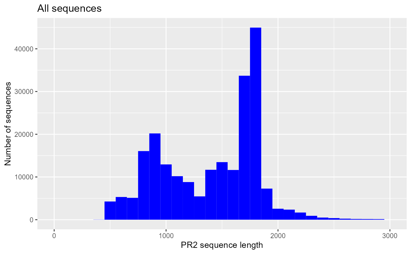
ggplot(pr2_ref) + geom_histogram(aes(sequence_length), binwidth = 100, fill="blue") +
  xlim(0,3000) +
  xlab("PR2 sequence length") +
  ylab("Number of sequences") +
  ggtitle("Reference sequences")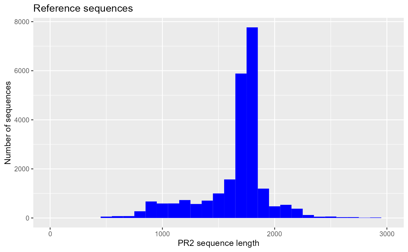
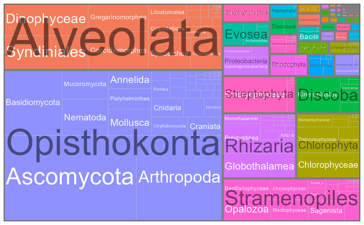
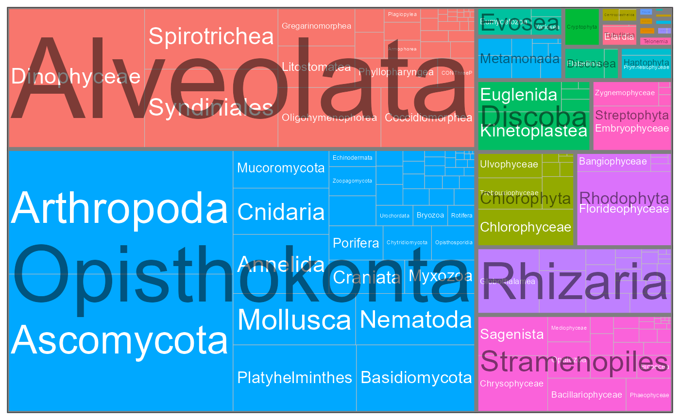
Taxonomic composition
pr2_treemap <- function(pr2, level1, level2) {


  # Group
  pr2_class <- pr2 %>%
    count({{level1}},{{level2}}) %>%
    filter(!is.na(division)) %>%
    ungroup()

  # Do a treemap

  ggplot(pr2_class, aes(area = n,
                        fill = {{level2}},
                        subgroup = {{level1}},
                        label = {{level2}})) +
           treemapify::geom_treemap()

  ggplot(pr2_class, aes(area = n,
                        fill= {{level1}},
                        subgroup = {{level1}},
                        label = {{level2}})) +
    treemapify::geom_treemap() +
    treemapify::geom_treemap_text(colour = "white", place = "centre", grow = TRUE) +
    treemapify::geom_treemap_subgroup_border() +
    treemapify::geom_treemap_subgroup_text(place = "centre", grow = T,
                                           alpha = 0.5, colour = "black",
                                           min.size = 0) +
    theme_bw() +
    scale_color_brewer() +
    guides(fill = FALSE)

}

Genera most represented
All taxa
pr2_genus <- pr2 %>% group_by(class, genus) %>%
  count() %>%
  ungroup() %>%
  top_n(30)

ggplot(pr2_genus) +
  geom_col(aes(x=forcats::fct_reorder(stringr::str_c(class,"-",genus), n), y=n)) +
  coord_flip() +
  ggtitle("Most represented genera - all") +
  xlab("Genera") + ylab("Number of sequences")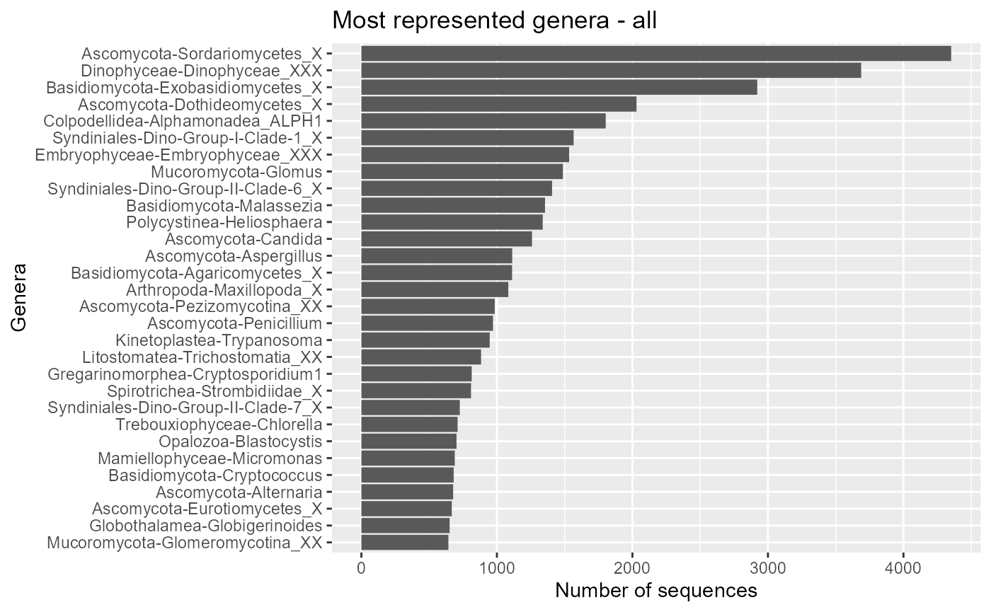
Reference sequences
pr2_genus <- pr2_ref %>%
  group_by(class, genus) %>%
  count() %>% ungroup() %>%
  top_n(30)

ggplot(pr2_genus) +
  geom_col(aes(x=forcats::fct_reorder(stringr::str_c(class,"-",genus), n), y=n)) +
  coord_flip() +
  ggtitle("Reference sequences") +
  xlab("Genera") +
  ylab("Number of sequences")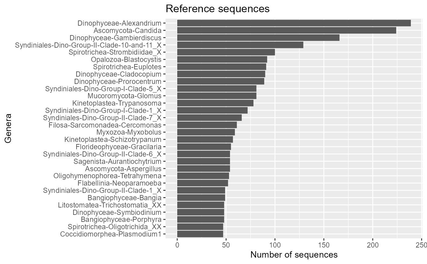
Only photosynthetic protists
  pr2_genus <- pr2_photo %>%
  group_by(class, genus) %>%
  count() %>%
  ungroup() %>%
  top_n(30)

  ggplot(pr2_genus) +
    geom_col(aes(x=forcats::fct_reorder(stringr::str_c(class,"-",genus), n), y=n)) +
    coord_flip() +
    ggtitle("Most represented genera - only photosynthetic protists") +
    xlab("Genera") + ylab("Number of sequences")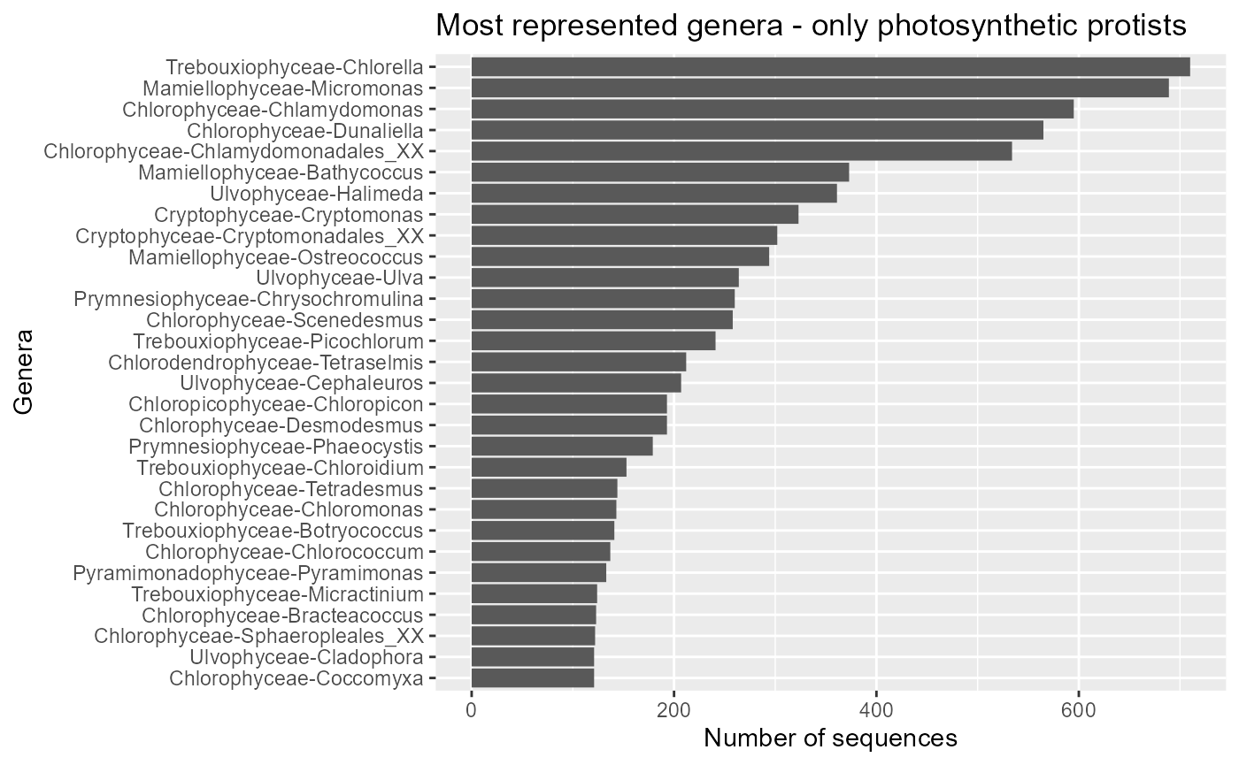
World sequence distribution
map_get_world <- function(resolution="coarse"){
  # Change to "coarse" for global maps / "low" for regional maps
  worldMap <- rworldmap::getMap(resolution = resolution)
  world.points <- fortify(worldMap)
  world.points$region <- world.points$id
  world.df <- world.points[,c("long","lat","group", "region")]
  }


map_world <- function(color_continents = "grey80",
                      color_borders = "white",
                      resolution = "coarse") {

  # Background map using the maps package
  # world.df <- map_data("world")

  world.df <- map_get_world(resolution)

  map <- ggplot() +
    geom_polygon(data = world.df,
                 aes(x=long, y = lat, group = group),
                 fill=color_continents,
                 color=color_borders) +
    # scale_fill_manual(values= color_continents , guide = FALSE) +
    scale_x_continuous(breaks = (-4:4) * 45) +
    scale_y_continuous(breaks = (-2:2) * 30) +
    xlab("Longitude") + ylab("Latitude") +
    coord_fixed(1.3) +
    theme_bw()
    # species_map <- species_map + coord_map ()  # Mercator projection
    # species_map <- species_map + coord_map("gilbert") # Nice for the poles
  return(map)
  }
All taxa
 map_world() + geom_point(data=pr2, aes(x=pr2_longitude, y=pr2_latitude),
                          fill="blue", size=2, shape=21) +
ggtitle("PR2 - all sequences") 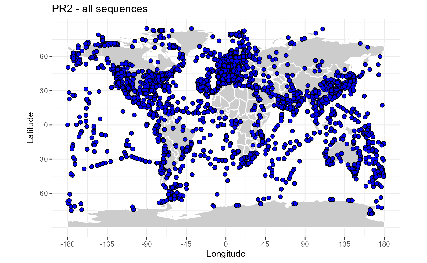
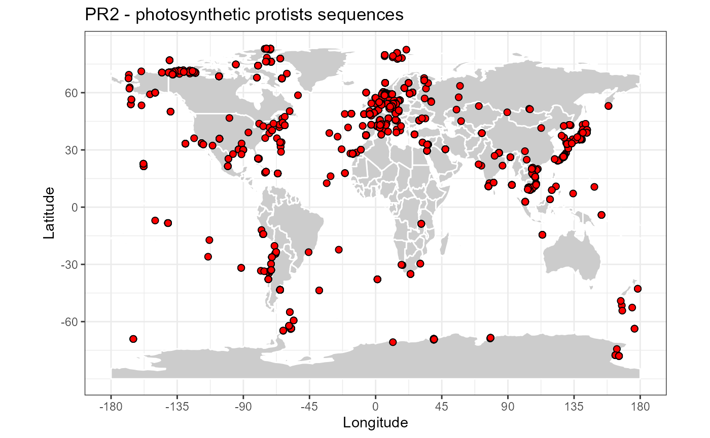
Photosynthetic protists
 map_world() + geom_point(data=pr2_photo, aes(x=pr2_longitude, y=pr2_latitude),
                          fill="red", size=2, shape=21) +
               ggtitle("PR2 - photosynthetic protists sequences")